From OpenStreetMap APIs to Insightful Data Analysis: Extraction, Analysis, and Mapping with R

State of the Map - Paris 2026

Louis Laurian, Timothée Giraud, Matthieu Viry, Ronan Ysebaert

Centre pour l’analyse spatiale et la géovisualisation

28 Aug 2026

Plan

• The R Software
• R and OSM
• Reproducible Example

In this talk we will talk about how it is possible to use OSM data and related from the statistical software R.

We have to explain our positionning first. We work for a research laboratory in CNRS. We use OSM data as input for scientific studies. For exemple we have work on interactions across French borders. We have also work intensively on accessibility to rural areas at european scale.

Doing so we use OSM data as is, as a primary source of raw data. So we do not contribute in anyway to the OSM data base (in the time spend at the office).

In order to use the data and tool in a profesional way we use a specific software (and language) made for and by researchers: the R software. To respond to some specific needs we had to extend the R software package ecosystem. We have developped some R package to interact with the OSM DB or some 3rd party tools.

In this talk we’ll start by introducing you to the R Software and its specificities, we’ll then present an opiniated list of OSM related R packages, we’ll finish with a comprehensive exemple that demonstrate how to use these package.

R

The R Software

• Free and open source software (GNU GPLv3)
• Work most OS
• Geared towards reproducible research
• Unified workflows
• Packages developed by the community (CRAN)

R stands out as a free and open source programming language and software for statistical computing and data visualization.

Complemented by more than 23,500 user-contributed packages hosted on the Comprehensive R Archive Network in 2026.

The language’s versatility allows users to build unified workflows within an environment conducive to reproducible research.

R is widely used for research purposes in many fields beyond statistics, such as biology, social sciences, or geomatics.

The R Software Spatial Ecosystem

Vector Data Handling

sf (Pebesma, 2018)

Main features

• import / export
• display
• geoprocessing
• support for unprojected data
• use of the simple feature standard

Raster Data Handling

terra (Hijmans, 2022)

Main features

• import / export
• display
• study area modifications
• spatial algebra
• transformation and conversion

A subset of R packages forms a robust and mature spatial ecosystem that makes it easy to handle and display spatial data.

The 2 main packages used to deal with spatial data are sf and terra. Both are base on GDAL, PROJ and PROJ to handle data import, projections and geoprocessing

The R Software Spatial Ecosystem

Thematic Cartography

mapsf (Giraud, 2023a)

tmap (Tennekes, 2018)

ggplot2 + ggspatial (Dunnington, 2025)

Spatial analysis / spatial statistics

• spatstat : Point pattern analysis
• gstat : Variograms and Krigeage
• rgeoda : Geoda with R
• GWmodel, spgwr : Geographically Weighted Models

CRAN Task View: Analysis of Spatial Data

• Spatial sampling
• Point pattern analysis
• Geostatistics
• Disease mapping and areal data analysis
• Spatial regression
• Ecological analysis

To complement this overview on the spatial ecosystem of the R software we can have a look at some package for thematic cartograhy.
mapsf is developped in our lab. It aims at creating thematic or statistitcal maps. tmap is an alternative to mapsf that use a different syntax, close to the one of the ggplot2 package that also allow to crate thematic maps.

At last, as a statistical programming language, R allows to use a lot of spatial analysis or spatial statistic computations. You have only a short overview of it.

R and OSM

R provides seamless access to various APIs and tools for downloading and filtering OpenStreetMap data, querying shortest routes and itineraries, or generating both static and interactive maps.

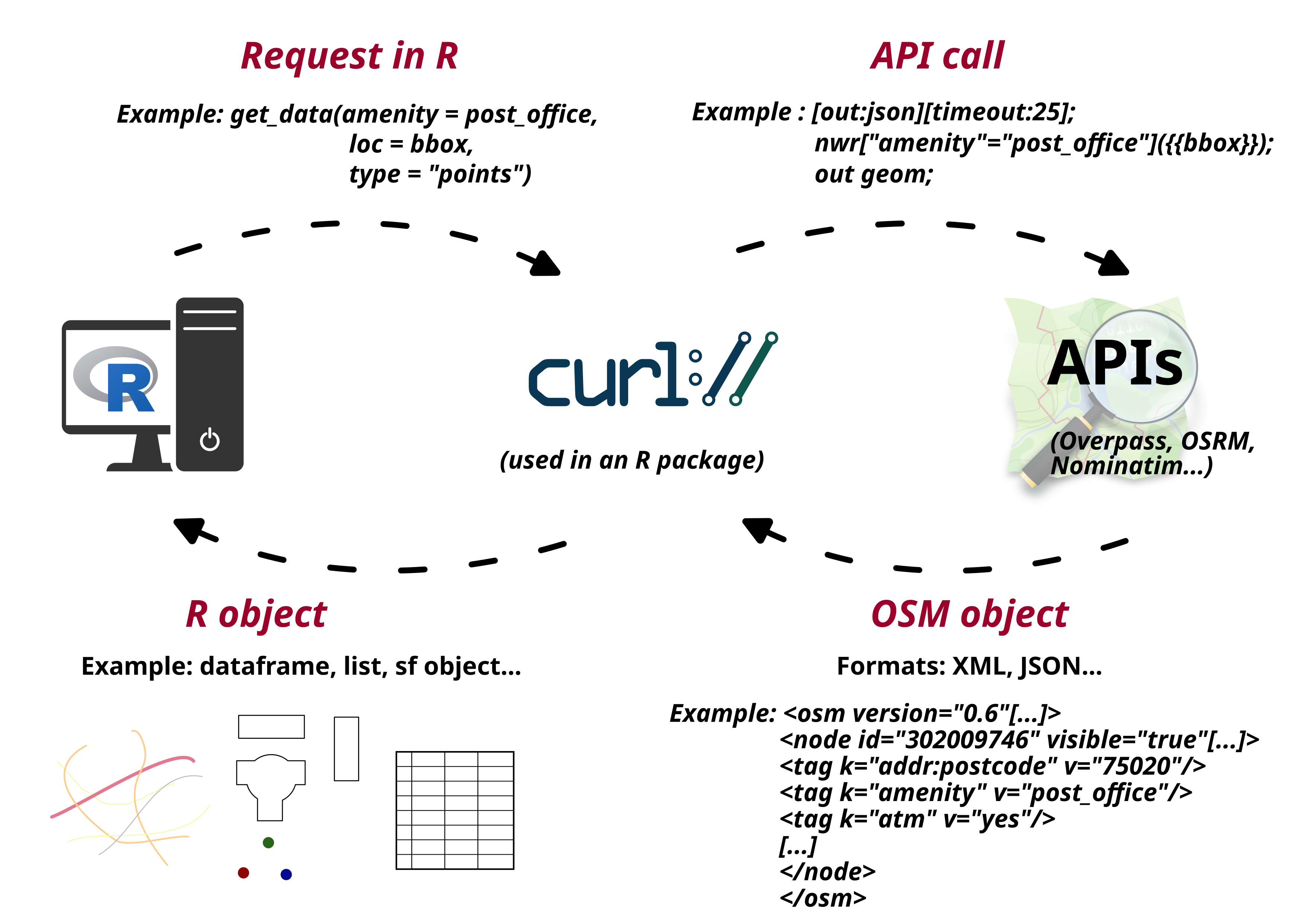
How does it work ?

Overview

Access to the database

Find OSM data

• Geofabrik download server

• BBBike

• Overpass API

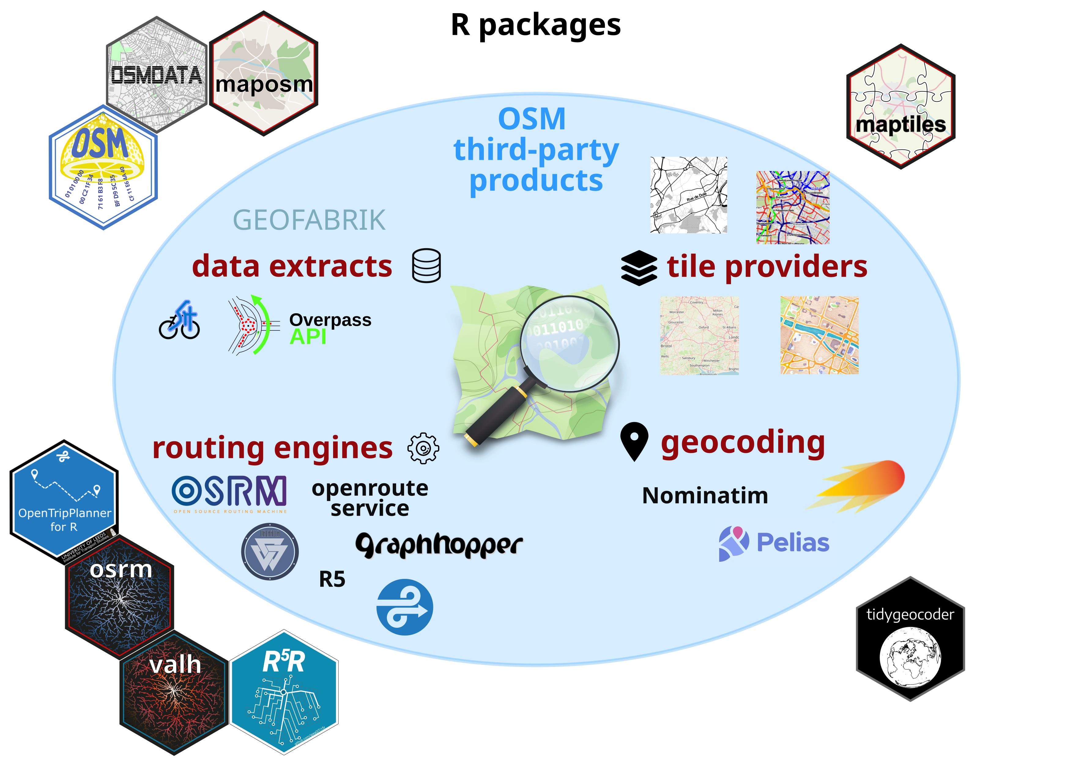
R packages

• osmextract (Gilardi and Lovelace, 2021), imports datasets from both Geofabrik and BBBike

• osmdata (Mark Padgham et al., 2017), downloads OSM data from the Overpass API

We begin with packages that download and extract data, such as osmextract and osmdata

Geocoding and Routing

Routing engines

• OSRM, pre-processed routes

• Valhalla, based on tiles

• R5, allows multimodal routing (GTFS tables)

• OpenTripPlanner, integrated web server

• Openrouteservice

• GraphHopper

Geocoding tools

• Nominatim

• Photon

• Pelias

R packages

• osrm (Giraud, 2022)

• valh (Giraud and Viry, 2025)

• r5r (Pereira et al., 2021)

• opentripplanner (Malcolm Morgan et al., 2019)

• tidygeocoder (Cambon et al., 2021), 15+ providers (default Nominatim)

we explore solutions that interface third party softwares for geocoding (Nominatim with tidygeocoder) and routing (OSRM with osrm, Valhalla with valh)

Cartography

OSM layers

• Tile providers

R packages

• leaflet (Cheng et al., 2018) and mapview (Appelhans et al., 2018), dynamic cartography (OSM background)

• maptiles (Giraud, 2023b), downloads raster tiles

• maposm (not yet on CRAN), downloads geographic layers

we address dynamic cartography (using leaflet) and creation of static maps from raster tiles (using maptiles) or from vector objects (using maposm)

Reproducible Example

To illustrate the practical application of these tools, we conclude with a short, seamless and fully reproducible example. From the geocoding of an address, to the extraction of amenities or the use of routing engines and till the creation of a publication-ready map, we propose a complete workflow that harness the power of R ecosystem to create insightful analysis from OpenStreetMap data.

Geocoding - Retrieve coordinates from an address

library(sf) # for spatial data processing
library(tidygeocoder) # geocoding

# SOTM 2026 address
pt <- geo(address = "6 Av. Blaise Pascal, 77420 Champs-sur-Marne", method = "osm")
# Transform dataframe with X/Y coords to an sf object
(pt <- st_as_sf(pt, coords = c("long", "lat"), crs = 4326))

Simple feature collection with 1 feature and 1 field
Geometry type: POINT
Dimension:     XY
Bounding box:  xmin: 2.587371 ymin: 48.84108 xmax: 2.587371 ymax: 48.84108
Geodetic CRS:  WGS 84
# A tibble: 1 × 2
  address                                                geometry
* <chr>                                               <POINT [°]>
1 6 Av. Blaise Pascal, 77420 Champs-sur-Marne (2.587371 48.84108)

Interactive map with OSM background layer

library(mapview)
mapview(pt, map.types = "OpenStreetMap.Mapnik")

Tiles extraction - Raster format

library(maptiles)
# Define a bounding box around our address
bbox <- st_bbox(st_buffer(pt, 500))
# Download tiles covering the bounding box
tiles <- get_tiles(x = bbox, project = FALSE,
                   provider = "OpenStreetMap.HOT",
                   zoom = 16, crop = TRUE)
tiles

class       : SpatRaster
size        : 644, 644, 3  (nrow, ncol, nlyr)
resolution  : 2.388657, 2.388657  (x, y)
extent      : 287257.5, 288795.8, 6247172, 6248710  (xmin, xmax, ymin, ymax)
coord. ref. : WGS 84 / Pseudo-Mercator (EPSG:3857)
source      : tiles.tif
colors rgb  : 1, 2, 3
names       : red, green, blue
min values  :  82,    82,   82
max values  : 255,   255,  255

Plot tiles - Raster format

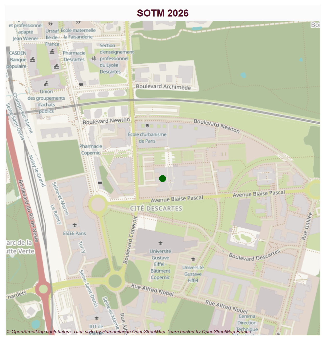
library(mapsf)
pt <- st_transform(pt, 3857)
mf_raster(tiles)
mf_map(pt, col = "darkgreen", cex = 3, add = TRUE)
mf_credits(maptiles::get_credit("OpenStreetMap.HOT"))
mf_title("SOTM 2026")

Download OSM data - from Overpass API

library(osmdata)
poi <- bbox |> 
  opq(osm_types = "node") |>
  add_osm_feature(key = 'amenity', value = "post_office") |>
  osmdata_sf()
po <- poi$osm_points
flextable::flextable(po, col_keys = names(po))

osm_id	name	addr:city	addr:housenumber	addr:postcode	addr:street	amenity	atm	change_machine	copy_facility	opening_hours	operator	operator:wikidata	panoramax	phone	post_office	ref:FR:LaPoste	source	stamping_machine	website	wheelchair	geometry
813539238	La Poste	Champs-sur-Marne	5	77420	Avenue André-Marie Ampère	post_office	yes	yes	yes	Mo-Fr 13:45-18:00; Sa 09:00-12:00; PH off; 2024 May 20 off	La Poste	Q373724	c7f797ac-9540-4f6c-9f7e-fa38de9f7718	3631	bureau	14675A	data.gouv.fr:LaPoste - 06/2015	yes	https://www.laposte.fr/	yes	[[XY]]

Download OSM data - from Overpass API

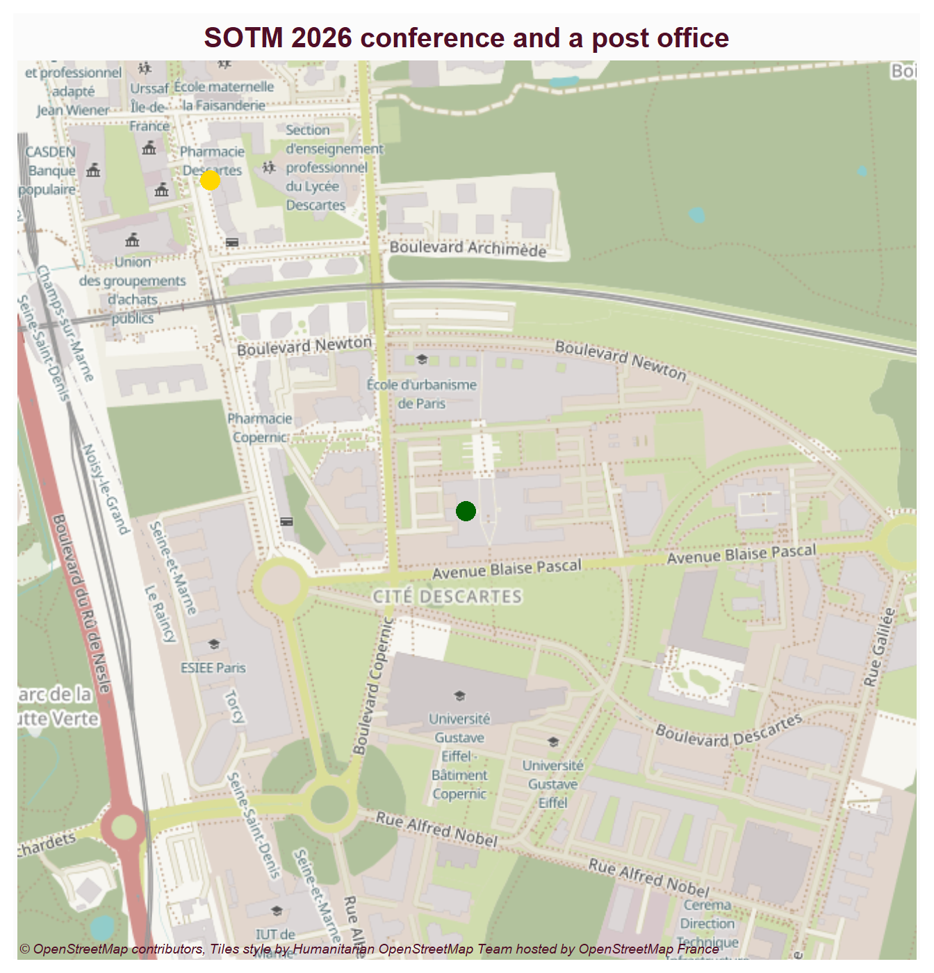
po <- st_transform(po[1,], 3857)
mf_raster(tiles)
mf_map(pt, col = "darkgreen", cex = 3, add = TRUE)
mf_map(po, col = "gold1", cex = 3, add = TRUE)
mf_credits(maptiles::get_credit("OpenStreetMap.HOT"))
mf_title("SOTM 2026 conference and a post office")

Routing - interface OSRM and Valhalla APIs

library(osrm)
library(valh)
# Shortest route from the address to the first post office
road_o <- osrmRoute(src = pt, dst = po, osrm.profile = "bike")
road_v <- vl_route(src = pt, dst = po, costing = "bicycle")
road_o
road_v

Simple feature collection with 1 feature and 4 fields
Geometry type: LINESTRING
Dimension:     XY
Bounding box:  xmin: 287553.8 ymin: 6247937 xmax: 287981.3 ymax: 6248507
Projected CRS: WGS 84 / Pseudo-Mercator
            src       dst duration distance                       geometry
1_813539238   1 813539238 3.913333   0.6437 LINESTRING (287981.3 624793...

Simple feature collection with 1 feature and 4 fields
Geometry type: LINESTRING
Dimension:     XY
Bounding box:  xmin: 287554.6 ymin: 6247940 xmax: 288057.1 ymax: 6248498
Projected CRS: WGS 84 / Pseudo-Mercator
            src       dst duration distance                       geometry
1_813539238   1 813539238  2.81915    0.673 LINESTRING (288048.5 624794...

Map the results

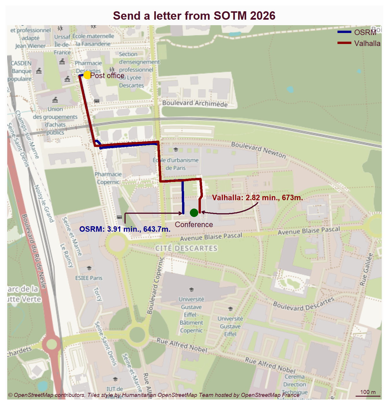
road_o <- st_transform(road_o, 3857)
road_v <- st_transform(road_v, 3857)
start_o <- st_cast(road_o, "POINT")[1,]
start_v <- st_cast(road_v, "POINT")[1,]
mf_raster(tiles)
mf_map(road_o, col = "darkblue", lwd = 4, add = TRUE)
mf_map(road_v, col = "darkred", lwd = 4, add = TRUE)
mf_map(pt, col = "darkgreen", cex = 3, add = TRUE)
mf_map(po, col = "gold1", cex = 3, add = TRUE)
mf_title("Send a letter from SOTM 2026")
mf_scale(100, scale_units = "m")
mf_credits(maptiles::get_credit("OpenStreetMap.HOT"))
mf_legend(type = "typo_line", pos = "topright",
          val = c("OSRM", "Valhalla"),
          pal = c("darkblue", "darkred"),
          lwd = 4, val_cex = .8, title = NA)
mf_text(x = pt, txt = "Conference", pos = "bottom",
        offset = 2)
mf_text(x = po, txt = "Post office", pos = "right")
mf_text(x = start_o, col_txt = "darkblue", cex = .8,
        pos = "bottomleft", line = 2, clockwise = TRUE,
        offset = 5,font = 2, txt = paste0("OSRM: ",
        round(road_o$duration,2), " min., ",
        road_o$distance * 1000, "m."))
mf_text(x = start_v, col_txt = "darkred", cex = .8,
        pos = "topright", line = 3, clockwise = TRUE,
        offset = 5, font = 2, txt = paste0(
          "Valhalla: ", round(road_v$duration,2),
          " min., ", road_v$distance * 1000, "m."))

And now for the reproducibility…

Throwback to last year

pt <- geo(address = "GT-Toyota Asian Center Auditorium, Magsaysay Avenue",
          method = "osm")
pt <- st_as_sf(pt, coords = c("long", "lat"), crs = 4326)
bbox <- st_bbox(st_buffer(pt, 500))
tiles <- get_tiles(x = bbox, project = FALSE,
                   provider = "OpenStreetMap.HOT",
                   zoom = 16, crop = TRUE)
pt <- st_transform(pt, 3857)
poi <- bbox |> 
  opq(osm_types = "node") |>
  add_osm_feature(key = 'amenity', value = "post_office") |>
  osmdata_sf()
poi <- poi$osm_points
po <- st_transform(poi[1,], 3857)
road_o <- osrmRoute(src = pt, dst = po, osrm.profile = "bike")
road_v <- vl_route(src = pt, dst = po, costing = "bicycle")
road_o <- st_transform(road_o, 3857)
road_v <- st_transform(road_v, 3857)
start_o <- st_cast(road_o, "POINT")[1,]
start_v <- st_cast(road_v, "POINT")[1,]
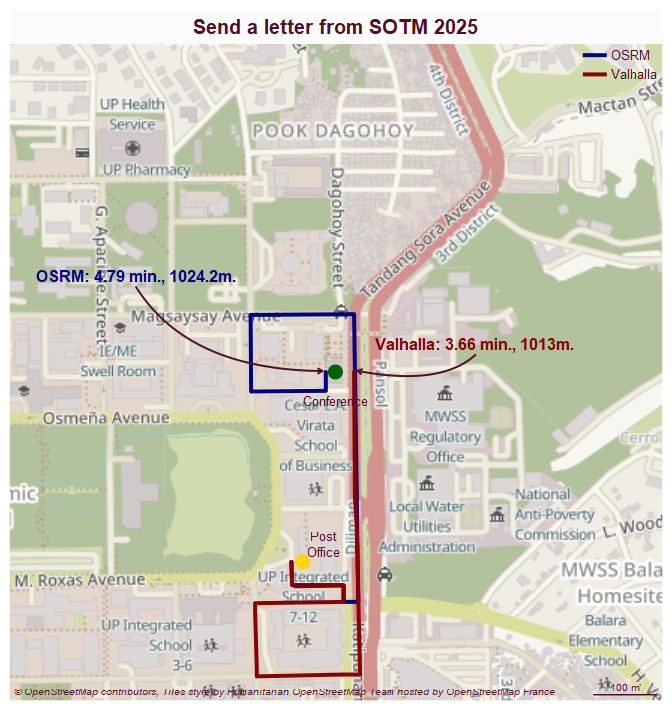
mf_raster(tiles)
mf_map(road_o, col = "darkblue", lwd = 4, add = TRUE)
mf_map(road_v, col = "darkred", lwd = 4, add = TRUE)
mf_map(pt, col = "darkgreen", cex = 3, add = TRUE)
mf_map(po, col = "gold1", cex = 3, add = TRUE)
mf_title("Send a letter from SOTM 2025")
mf_scale(100, scale_units = "m")
mf_credits(maptiles::get_credit("OpenStreetMap.HOT"))
mf_legend(type = "typo_line", val = c("OSRM", "Valhalla"),
          pal = c("darkblue", "darkred"), pos = "topright",
          lwd = 4, val_cex = .8, title = NA)
mf_text(x = pt, txt = "Conference", pos = "bottom", offset = 2)
mf_text(x = po, txt = "Post\nOffice", pos = "topright")
mf_text(x = start_o, col_txt = "darkblue", pos = "topleft", 
        cex = 1, line = 3, clockwise = FALSE, offset = 25, font = 2,
        txt = paste0("OSRM: ", round(road_o$duration,2),
                     " min., ", road_o$distance * 1000, "m."))
mf_text(x = start_v, col_txt = "darkred", pos = "topright", 
        cex = 1, line = 3, clockwise = TRUE, offset = 5, font = 2,
        txt = paste0("Valhalla: ", round(road_v$duration,2),
                     " min., ", road_v$distance * 1000, "m."))

Examples of RIATE’s work with OSM data

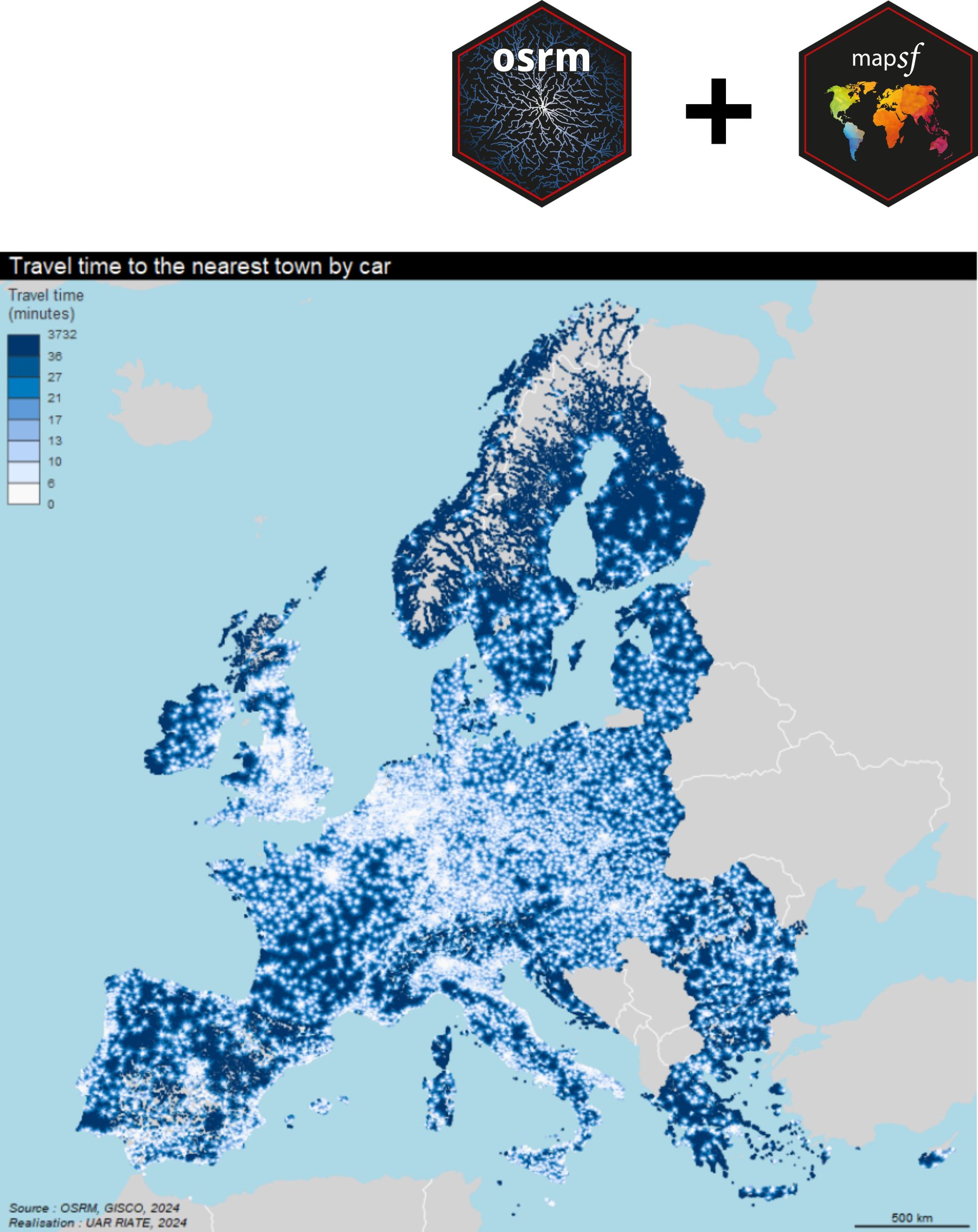
Accessibility indicators at EU scale (2024)

Cartographic exploration of the OSM database with R (2018)

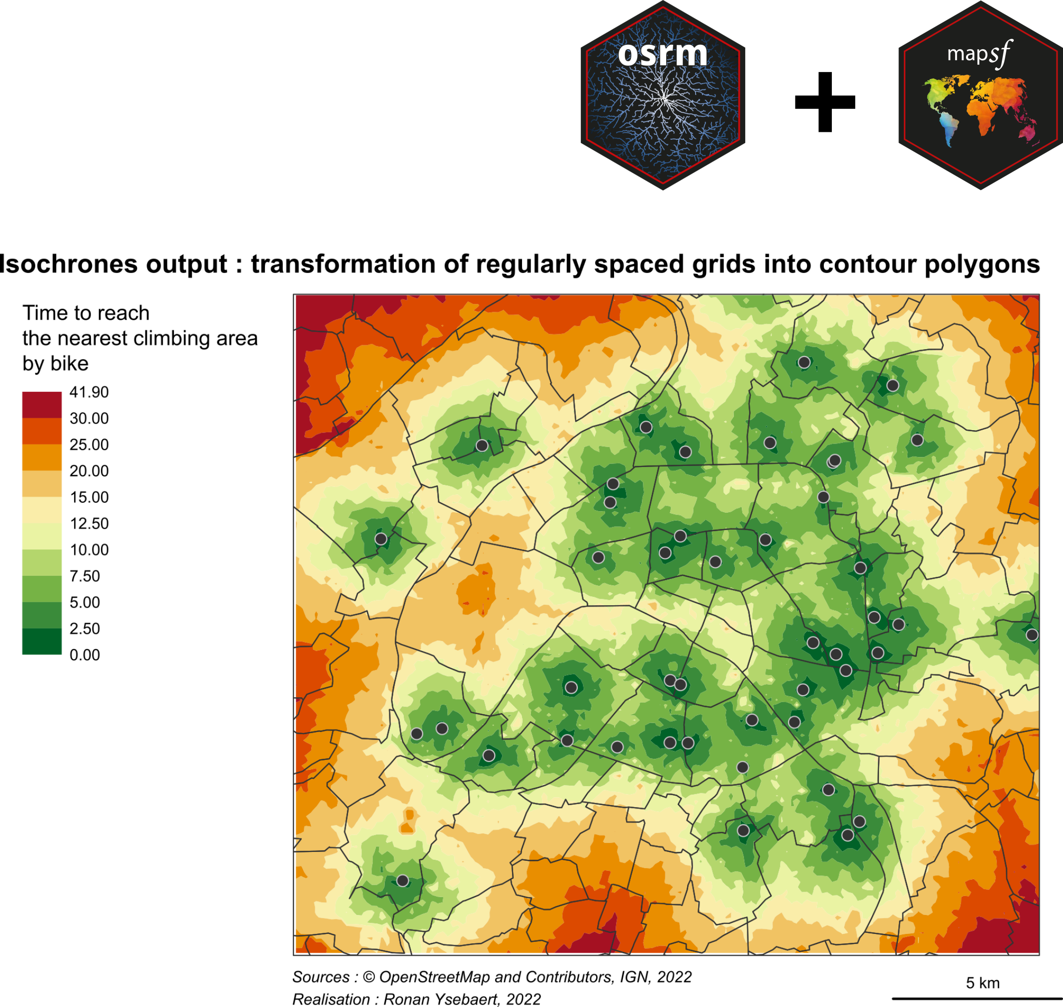
Accessibility to climbing walls in Paris (2023)

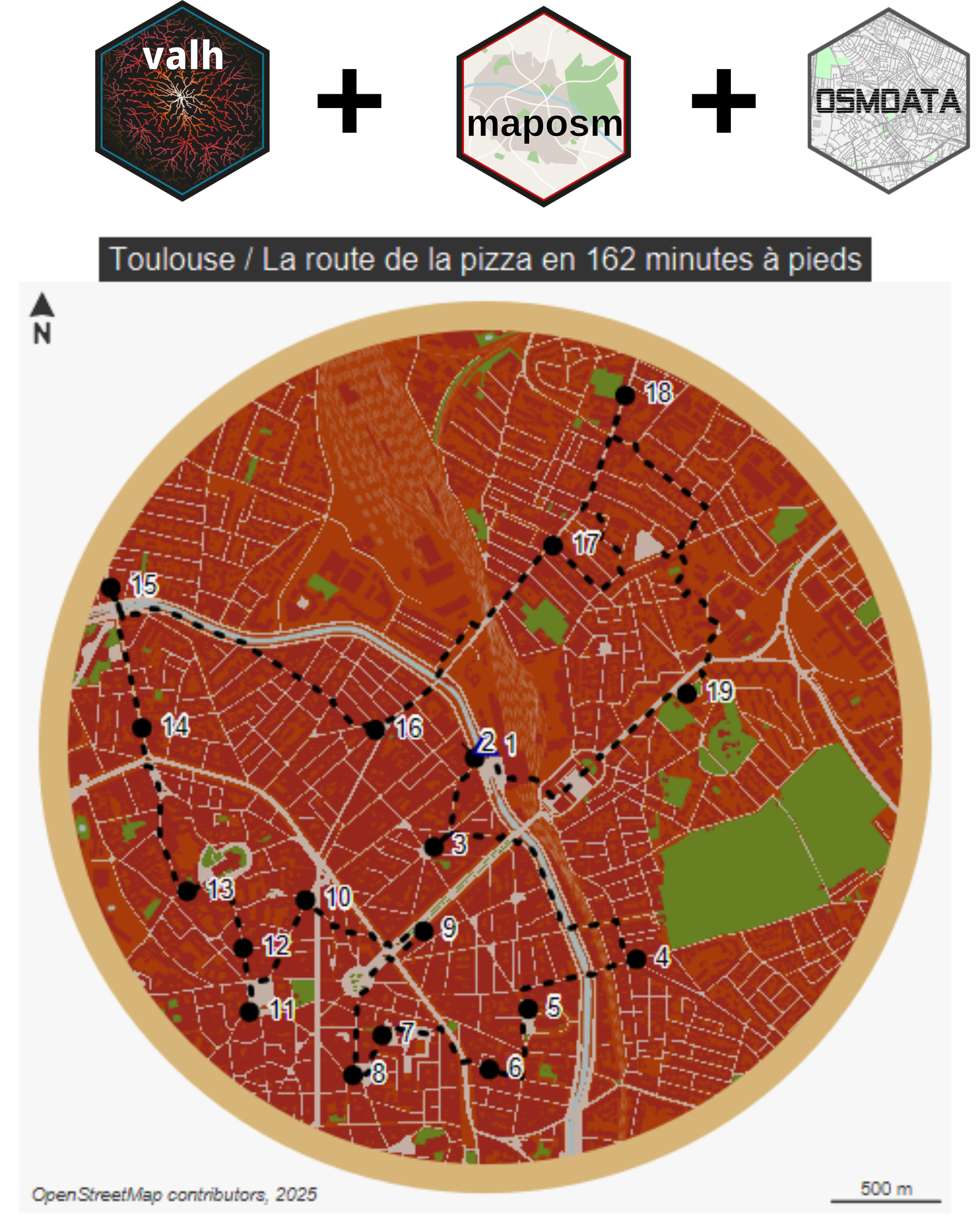
Utiliser OpenStreetMap avec R (2025)

Bonus

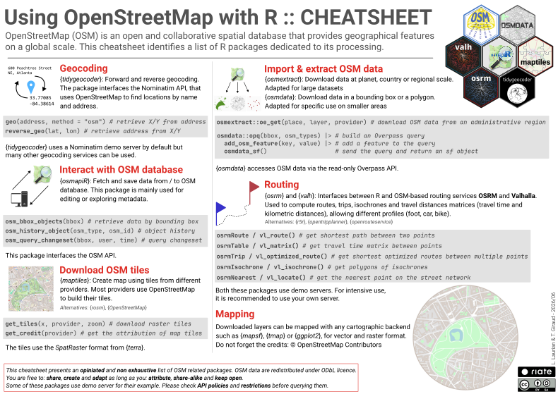
Using OSM with R, the cheat sheet

Cheat sheets are a common documentation format for R packages. We’ve built this cheat sheet to give and overview of what is possible to do with OSM from R. The first page describes the main functions of the main packages related to OSM. Packages are organised by theme.

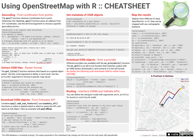
Using OSM with R, the cheat sheet

You can download the cheat sheet using the QR code:

https://zenodo.org/records/20842874

The cheat sheet is hosted on Zenodo, you can use the following QR code to access the page or use the link.

Thank you

You can access the slides using the QR code:

https://riatecom.github.io/R_OSM_SOTM_2026/

You can access the slides using the QR code or with the link on screen.

References

Appelhans, T., Detsch, F., Reudenbach, C. and Woellauer, S. (2018). Mapview: Interactive viewing of spatial data in r. https://github.com/r-spatial/mapview

Cambon, J., Hernangómez, D., Belanger, C. and Possenriede, D. (2021). Tidygeocoder: An r package for geocoding. Journal of Open Source Software, 6(65), 3544. https://doi.org/10.21105/joss.03544

Cheng, J., Schloerke, B., Karambelkar, B., Xie, Y. and Aden-Buie, G. (2018). Leaflet: Create interactive web maps with the JavaScript ’leaflet’ library. https://rstudio.github.io/leaflet/

Dunnington, D. (2025). Ggspatial: Spatial data framework for ggplot2. https://doi.org/10.32614/CRAN.package.ggspatial

Gilardi, A. and Lovelace, R. (2021). Osmextract: Download and import open street map data extracts. https://doi.org/10.32614/CRAN.package.osmextract

Giraud, T. (2022). osrm: Interface Between R and the OpenStreetMap-Based Routing Service OSRM. Journal of Open Source Software, 7(78), 4574. https://doi.org/10.21105/joss.04574

Giraud, T. (2023a). mapsf: Thematic cartography. https://doi.org/10.32614/CRAN.package.mapsf

Giraud, T. (2023b). Maptiles: Download and display map tiles. https://doi.org/10.32614/CRAN.package.maptiles

Giraud, T. and Viry, M. (2025). Valh: Interface between r and the OpenStreetMap-based routing service valhalla. https://doi.org/10.32614/CRAN.package.valh

Hijmans, R. J. (2022). Terra: Spatial data analysis. https://doi.org/10.32614/CRAN.package.terra

Malcolm Morgan, Marcus Young, Robin Lovelace and Layik Hama. (2019). OpenTripPlanner for r. Journal of Open Source Software, 4(44), 1926. https://doi.org/10.21105/joss.01926

Mark Padgham, Bob Rudis, Robin Lovelace and Maëlle Salmon. (2017). Osmdata. Journal of Open Source Software, 2(14), 305. https://doi.org/10.21105/joss.00305

Pebesma, E. (2018). Simple Features for R: Standardized Support for Spatial Vector Data. The R Journal, 10(1), 439–446. https://doi.org/10.32614/RJ-2018-009

Pereira, R. H. M., Saraiva, M., Herszenhut, D., Braga, C. K. V. and Conway, M. W. (2021). r5r: Rapid realistic routing on multimodal transport networks with R\(^{\textrm{5}}\) in r. Findings. https://doi.org/10.32866/001c.21262

Tennekes, M. (2018). tmap: Thematic maps in R. Journal of Statistical Software, 84(6), 1–39. https://doi.org/10.18637/jss.v084.i06